One-step generative models

I have been spending a lot of time on one-step generative models, specifically MeanFlow and the broader family it belongs to. This is my attempt to build an honest mental model of how these methods work, where the math comes from, and how each one is a response to the limitations of the one before it.

The context: diffusion and flow models can now produce images, audio, and video that are nearly indistinguishable from real data, but generating a single sample requires hundreds of sequential network evaluations. That is fine for offline synthesis. It is nearly unusable for anything interactive or real-time. The last two years have seen a serious push to fix this, and the results are surprisingly good.

Starting from the goal and working backwards: what does a network need to learn to generate in one step?

Generation as transport

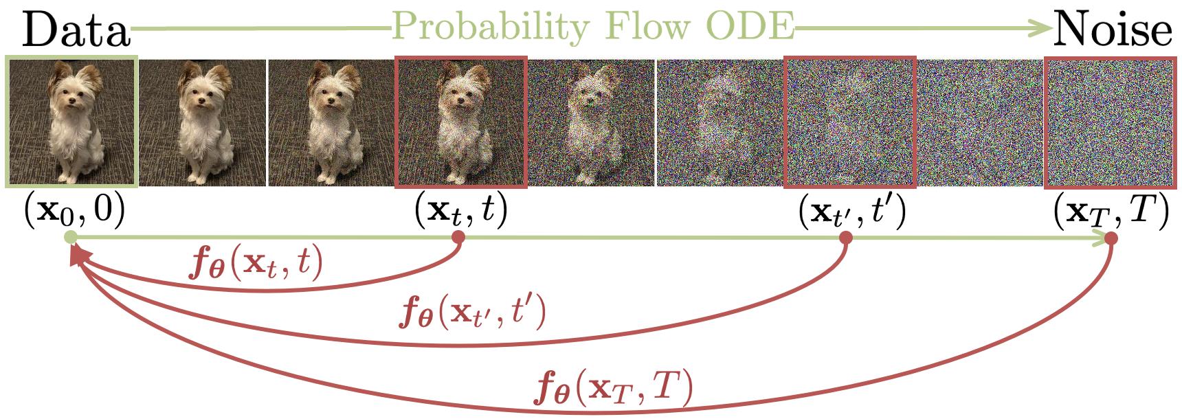
Generating a sample is moving probability mass from a noise distribution to the data distribution, and every method in this family is a different way to learn that movement. They all share the same setup: a trajectory through image space, a path from pure noise at time $t=1$ to clean data at time $t=0$. This is the probability flow ODE (PF-ODE), a deterministic path that shares the same marginal distributions at each time $t$ as the stochastic diffusion process but without the randomness. You can run it forwards or backwards exactly.

Think of a soap bubble. Press it slowly and the surface deforms; every point on the film follows a smooth, deterministic path. Release the pressure and it snaps back along the exact same path, not an approximation. The PF-ODE is that elastic surface in probability space: a deterministic velocity field that moves every point from noise to data (or back) along a reversible path, with no randomness. A point $z_t$ on a trajectory is one spot on that surface at time $t$.

The closer $t$ is to 1, the more spread out and featureless the point. The PF-ODE tells you how fast and in which direction to move to stay on the trajectory, and standard diffusion and flow models learn to estimate this velocity locally and integrate it step by step from noise to data.

The core problem with step-by-step integration: the local velocity at $z_t$ tells you nothing about where the trajectory ends up globally. You have to follow it closely, one small step at a time, or you drift off course and end up somewhere wrong. This is expensive.

Two strategies for escaping this:

1. Jump to the endpoint directly. Learn a function that maps any trajectory point to $x_0$ in one shot. This is the consistency model idea.
2. Jump to any point, not just the endpoint. Learn a two-time function that can jump from any $t$ to any $s < t$ in one step. This is the flow map idea, and it is what CTM, shortcut models, and MeanFlow (all coming up) build on.

Flow matching

Before getting to one-step methods, it helps to understand flow matching, because all the one-step methods either build on it or borrow its training structure. Flow matching ^[1] frames generation as transport: learn a continuous-time flow that moves probability mass from one distribution to another. The source and destination can be any two distributions; unlike diffusion models, you are not committed to Gaussian noise on one end. In practice, the simplest useful case uses Gaussian noise as the source, giving straight-line paths between noise and data:

The velocity at any point on this path is constant: $v = x_0 - x_1$. This is directly computable from training pairs, no score estimation, no self-referential structure. You train a network to predict this velocity at every $(z_t, t)$, which is just supervised regression on a clean ground-truth target.

Why is inference still slow? Even though each individual path $x_0 \leftrightarrow x_1$ is a straight line, the marginal velocity field is not. At any given noisy image $z_t$, many different clean images $x_0$ are plausible, not just one. Each candidate has its own straight-line velocity pointing in a slightly different direction. The network has to output the probability-weighted average of all those directions, which traces a curved path through image space. Following a curved path with only local velocity information requires many small steps.

Scrub the demo below to watch this happen: at $t=1$ the field points toward the centroid (no cluster has been chosen), and as $t$ decreases the weights concentrate and particles fan out toward different clusters. Try the candidates buttons (1, 3, 5) to see how a single cluster gives a uniform field while multiple clusters force curvature.

Flow matching gives you clean, stable training but slow inference. Every method we discuss next is trying to fix the inference speed without giving up that training clarity.

Consistency models

Consistency models ^[2] were the first serious attempt at fixing the inference problem. Rather than learn the velocity and integrate it, learn a function that maps any point on the trajectory directly to the clean endpoint $x_0$:

Apply this once from pure noise, and you get a clean image. The model should give the same clean answer from any point on the same trajectory. Same idea as the equation above, drawn along one trajectory:

same trajectory:

noise side                         clean side
z_T  ─────── z_t ─────── z_s ─────── x_0

f_θ(z_T, T) → x_0
f_θ(z_t, t) → x_0
f_θ(z_s, s) → x_0
f_θ(x_0, 0) → x_0

For this to actually work, the function needs two properties. First, the boundary condition: at $t = 0$ (or more precisely, a small cutoff $\varepsilon$ near zero), the function must be the identity, $f_\theta(x_0, \varepsilon) = x_0$. A completely clean image maps to itself. Without it, the network could satisfy the rest of the loss by outputting a constant; the boundary condition pins one end of the function to something meaningful.

Second, the consistency condition: any two points on the same PF-ODE trajectory must map to the same $x_0$. If two different noisy versions of the same clean image both pass through the network, they should produce identical outputs. This is the key constraint that makes the function globally coherent rather than just locally trained. The figure below shows what this looks like: every point along one trajectory is required to map to the same destination.

How do you actually build $f_\theta$ so the boundary identity $f_\theta(x_0, \varepsilon) = x_0$ holds? The naive way is piecewise: define $f_\theta(x, t) = x$ when $t = \varepsilon$ and $f_\theta(x, t) = F_\theta(x, t)$ otherwise, where $F_\theta$ is a free neural network. This works for the discrete-time loss but breaks the moment you want continuous-time training, because the function is not differentiable at $\varepsilon$ and the continuous-time loss requires a clean derivative through $f_\theta$.

The fix the paper actually uses, and the one that has stuck, is to wire the boundary identity into the architecture algebraically with a skip / output split:

At $t = \varepsilon$ the formula collapses to $f_\theta(x, \varepsilon) = 1 \cdot x + 0 \cdot F_\theta = x$. The boundary condition is true by construction; the loss never has to enforce it. Crucially, because $c_\text{skip}$, $c_\text{out}$, and $F_\theta$ are all differentiable in $t$, so is $f_\theta$. That smoothness is what unlocks continuous-time consistency training, where the loss involves a derivative of $f_\theta$ with respect to $t$.

The specific functional forms for $c_\text{skip}$ and $c_\text{out}$ are inherited directly from the EDM diffusion preconditioning ^[10], which is a deliberate choice: it lets consistency models drop into existing diffusion architectures with no structural changes, just a different head and loss.

Enforcing consistency via self-distillation

Here is the problem: you never directly observe which trajectory any $z_t$ belongs to. You cannot enumerate all the $(z_t, z_s)$ pairs that should agree. What you can do is take two adjacent points on the same trajectory, $z_t$ and $z_{t-\Delta}$ separated by a small step, and ask that their predictions agree:

The EMA copy $\theta^-$ is updated slowly after each training step, typically $m \approx 0.99$, so the target moves at roughly 1% of the speed of the main network. This keeps the target stable enough to learn against. Without it, both sides of the loss update simultaneously and they can easily converge to the same wrong answer: outputting a constant everywhere, which technically satisfies the loss but is completely useless for generation.

The stop-gradient on the target side breaks this symmetry. Gradients only flow through the left side of the loss, so only $\theta$ is updated to chase the target. The target then drifts slowly via the EMA rule. This is the same target network trick from deep RL; it is what makes self-distillation stable.

To get the adjacent point $z_{t-\Delta}$ on the same trajectory as $z_t$, you need to take one step of the PF-ODE. This is where the teacher and student framing becomes explicit. In consistency distillation (CD), a pretrained diffusion model acts as the teacher: it provides reliable one-step ODE moves that land on the true trajectory, and the student learns to jump directly to $x_0$ from any point on those teacher-generated trajectories. In consistency training (CT), there is no external teacher; the network estimates the score from scratch and generates its own training pairs, which introduces additional noise and makes training harder to stabilise. CD is faster to converge and produces better results; CT avoids the dependency on a pretrained teacher at the cost of more careful engineering.

Worth pinning down the language here, because three different things in this post all get called “teacher” at various points and they are not the same. Data supervision means clean targets read directly from training pairs, like flow matching’s $v = x_0 - x_1$. A pretrained teacher is an external network trained separately, used in CD and later in AYF; quality is capped at whatever the teacher can do. The EMA copy $\theta^-$ is the network’s own slowly-moving lag of itself, used in CT, CTM, Shortcut, and the consistency half of MeanFlow. CT and CD differ exactly in this: CT has only the EMA copy, CD has both. From here on I will say “EMA copy” when I mean the internal lag and “pretrained teacher” when I mean a separately trained network.

The discretisation curriculum

There is one subtlety about consistency model training that matters. You divide the time axis into $N$ discrete steps. Adjacent training pairs are always one step apart, so the gap $\Delta = T/N$.

If $N$ is small, the gap is large. The two adjacent points are far apart on the PF-ODE trajectory. The training signal is strong (there is a lot of distance between the two predictions to align) but the targets are noisy. Taking a large step along the PF-ODE introduces large discretisation error, so $z_{t-\Delta}$ is only approximately on the right trajectory. You are training the network to agree with a somewhat wrong target.

If $N$ is large, the gap is small. The targets are very accurate (a tiny ODE step is nearly exact) but the training signal is weak. The two adjacent points are so close that their predictions are already similar. The loss gradient is tiny and training makes almost no progress.

Neither extreme works. The fix is a curriculum: start with small $N$ (coarse, strong signal, rough targets), then progressively increase $N$ (fine, weak signal, accurate targets). The network first learns a rough consistency function, then refines it. Slide $N$ in the demo below to see the tradeoff: at $N=1$ the Euler step from $z_t$ falls far off the true curve (large red gap, strong gradient); at $N=8$ it tracks the curve closely but the gradient barely moves the network.

Discrete-time vs continuous-time

What I described above is the discrete-time formulation: pick a grid of $N$ noise levels, define adjacent pairs on that grid, and run the curriculum on $N$. The grid is a crutch. It exists because we cannot directly enforce the consistency condition over a continuum, only at sampled pairs of points. The whole curriculum on $N$ is just managing the bias-variance tradeoff that the grid introduces.

The continuous-time formulation removes the grid entirely. Differentiating the consistency condition $f(z_t, t) = f(z_{t-\Delta}, t-\Delta)$ as $\Delta \to 0$ gives a PDE-style identity: $\partial_t f + v(z_t, t) \cdot \partial_z f = 0$ along the PF-ODE. The training loss enforces this identity at sampled $(z_t, t)$ pairs, no adjacent point needed, no grid to schedule. sCT and sCD ^[9] use this formulation and produce sharper results than the discrete-time version, because the bias from finite $\Delta$ is gone. The cost is a Jacobian-vector product (JVP) through the network to compute $\partial_z f \cdot v$, a single forward pass with forward-mode autodiff. Keep this trick in mind: MeanFlow, which we will get to later, uses essentially the same machinery for a different purpose.

Consistency models prove the point: you can generate decent images in one step. That was not obvious before 2023. iCT ^[3] improved substantially over the original with pseudo-Huber losses, a lognormal noise schedule, and progressive discretisation step doubling, but even these required considerable engineering effort just to be reliable.

The training target is always behavioural: it constrains what the network outputs at adjacent pairs of points, not what the underlying field should be. There is no ground truth for $f(z_t, t)$ that exists independently of the network. The optimal function is defined only implicitly, via the consistency condition and boundary condition, and can only be learned by having the network agree with itself across adjacent pairs. This is inherently noisy and sensitive to hyperparameters.

The deeper limitation: consistency models are stuck. They can only jump to one destination, the endpoint $x_0$. The function signature is $f(z_t, t) = x_0$; you tell it where you are and what time it is, and it predicts the endpoint. You cannot ask it to jump to an intermediate point. Multi-step generation therefore requires running the network multiple times and renoising between each evaluation, a clunky workaround that does not actually use the trajectory structure. The natural next question: what if the jump function could land anywhere, not just $x_0$?

Consistency trajectory models: any-to-any jumps

CTM ^[4] generalises consistency models in one clean move. Recall the PF-ODE trajectory we defined: a path parameterised by time, running from noise at $t=1$ to data at $t=0$. Consistency models always jump to the end of that path. CTM removes that restriction and learns a function that can jump to any point along the PF-ODE, not just the endpoint:

This is the two-time function: a completely flexible jump operator. You can take large or small steps, jump to any intermediate point on the trajectory, and compose multiple jumps to refine a generation.

The key constraint that makes this well-posed is the semigroup property. If you jump from $t$ to some intermediate $u$, and then jump from $u$ to $s$, you should get the same result as jumping directly from $t$ to $s$:

Drag the split point $u$ in the figure below to see this in action: the direct jump (top arc) and the two-leg composition (bottom arcs) always end at the same destination, no matter where you split.

Training enforces this by sampling triples $(r, s, t)$ with $r < s < t$ and comparing the direct jump $G(x_t, t, r)$ against the composed two-step jump:

The flexible jump function makes multi-step generation more natural than consistency models: you chain calls with progressively smaller target times, no renoising needed. At the time of publication, CTM held the best single-step FID numbers (see the results table below).

The limitation it inherits from consistency models: the training target is still self-referential. $G_{\theta^-}$ is the network evaluated at a slightly lagged version of itself. There is no ground-truth two-time map that exists independently of the network; the only supervision comes from the model agreeing with itself across different decompositions. This makes training more stable than consistency models (because the semigroup structure is richer), but the fundamental self-referential nature remains. CTM is also fiddly in practice: random triples $(r, s, t)$, two separate network evaluations on the target side, careful coordination of all the moving parts. The methods that come next chip away at this complexity from different angles.

Shortcut models

Shortcut models ^[5] ask: what is the simplest possible way to enforce the semigroup property?

The answer: condition the network on both the current noise level $t$ and the desired step size $d$. The network learns to predict where you will end up after a jump of size $d$ from $z_t$. The step size is an input, not a fixed constant.

Think of it like this. A regular flow matching network only knows “I am at noise level $t$.” A shortcut model knows “I am at noise level $t$, and I want to travel a distance of $d$ in one step.” With that extra information, it can calibrate its prediction to the correct jump size and can be asked to take different step sizes at different points during generation.

The bootstrapping training procedure

How do you train this? You cannot compute the ground-truth $z_{t-d}$ directly, because it would require running the full ODE. The trick is to build the target out of smaller steps the network can already make. Two half-steps from the (stop-gradient) EMA copy of the network are composed into a single full-step target the student is trained to match. The picture first, equations after.

In equations, this is the semigroup property enforced discretely:

In practice, training starts with the smallest steps (where the half-step approximation is most accurate) and progressively learns larger steps using the smaller ones as building blocks. The network learns one-step jumps first, then two-step, then four-step, bootstrapping upward. At inference, you choose any step count: one for speed, many for quality.

Frans et al. draw the same construction with the actual loss notation overlaid; reproduced for cross-reference.

From the paper · Frans et al. 2024, Fig. 3

Shortcut models keep things simple by enforcing composition through direct comparison of network outputs: no differentiation through the network, no JVP, just a fast per-step training update. The tradeoff is that the discrete half-step approximation introduces small errors that compound when you compose many steps; and like CTM and consistency models before it, the training target is still self-referential. The next two methods both push against that self-reference. Align Your Flow does it by importing ground truth from outside (a pretrained teacher); MeanFlow does it from the inside (an exact identity that lets the network supervise itself against quantities readable directly from data).

Align Your Flow: distilling the jump function

Both CTM and Shortcut models work with the same flow-map object: a two-time network $f_\theta(x_t, t, s) = x_s$ that jumps from any noise level to any cleaner level in one forward pass. They train it from scratch with self-referential targets and pay for that with curriculum schedules and EMA copies of themselves on the target side. Align Your Flow ^[8] takes a different bet: instead of training the flow map from scratch, distill it from a pretrained diffusion teacher whose ODE trajectories are the ground truth.

From the paper · Sabour et al. 2025, Fig. 2

This framing resolves something that was implicit in CTM but never fully confronted. CTM trains the jump function so that composed shorter jumps reproduce longer ones, but it never asks whether the jump function is actually correct, only whether it is internally consistent. A pretrained teacher changes that: the teacher’s ODE trajectories are ground truth, and the student’s jumps are trained to trace them. Internal consistency is still enforced, but now there is an external anchor.

The paper also proves something sharp about consistency models. Theorem 3.1: for a Gaussian data source, even a suboptimal consistency model (and crucially, this holds for models arbitrarily close to optimal in $L_2$) admits some step count $N$ beyond which the Wasserstein-2 distance to the true distribution increases as you add more sampling steps. The empirical version is just as stark: with the standard EDM noise scale, CMs typically peak at around 2 steps and then degrade. The mechanism is specific. CMs jump to clean and renoise between steps; over many steps the reinjected noise does not align with the teacher’s PF-ODE trajectory and errors compound.

Flow maps avoid this by construction: they map directly between any two noise levels in one step, never leaving the trajectory. The paper does not formally prove they monotonically improve, but empirically they keep getting better with more steps, exactly where CMs fall apart.

Distilling the jump function from a teacher raises a practical question: how do you actually enforce the consistency constraint? AYF gives two answers, borrowing the fluid-dynamics distinction between Eulerian (fixed observer, watch the field) and Lagrangian (move with the particle) frames. The two losses differ in which time variable they perturb.

To replace classifier-free guidance during distillation, AYF uses autoguidance: the teacher is mixed with a weaker checkpoint of itself, $v_\phi^{\text{guided}} = \lambda v_\phi + (1 - \lambda) v_\phi^{\text{weak}}$ with $\lambda$ sampled uniformly from $[1, 3]$. This steers samples away from low-quality regions without the overshooting failure mode CFG can have.

The empirical headline (numbers are in the results table at the end): a small AYF student beats much larger distillation baselines at fewer NFEs. The efficiency gain comes from the teacher anchor: unlike CTM, the student does not waste capacity reconciling self-generated targets at high noise levels where those targets are most unreliable.

AYF resolves the self-referential issue by importing ground truth from outside (a teacher). The next method, MeanFlow, resolves it from the inside.

MeanFlow: ground truth for the jump function

MeanFlow ^[6] finds a quantity the network can predict whose true value is computable directly from data, no teacher required. That quantity is the average velocity.

Average velocity: a ground-truth two-time quantity

So what does “average velocity” actually mean here? It is the same thing it meant in physics class: total displacement divided by elapsed time. If you go from $z_t$ to $z_r$ over an interval of length $t - r$, the average velocity is just one divided by the other:

This looks unhelpful at first because $z_r$ is exactly the thing we cannot compute without integrating the ODE. But here is where flow matching does us a favor. Because the conditional paths are linear interpolations $z_t = (1-t)x_0 + tx_1$, the difference $z_t - z_r$ collapses algebraically:

That is the punchline. The average velocity is a fixed quantity for each training pair $(x_0, x_1)$, readable directly from data; no network evaluation, no self-reference, no approximation. And one-step generation falls out for free: start at pure noise, subtract the average velocity over the full interval, you have $x_0$.

The catch: this beautiful identity is only directly usable for the full interval $[0, 1]$ where you actually have ground-truth $(x_0, x_1)$ pairs. For arbitrary intermediate triples $(z_t, r, t)$ during training, computing $\bar{u}$ directly would require running the ODE, which is exactly what we are trying to avoid. The next subsection is how MeanFlow gets around that.

The MeanFlow identity

Computing $z_r$ requires running the PF-ODE from $z_t$ to time $r$, exactly the slow integration we are trying to avoid. MeanFlow gets around this by deriving an equivalent form that does not require $z_r$ at all. Start from the definition rewritten as an integral:

Now differentiate both sides with respect to $t$. The right side uses the fundamental theorem of calculus; the left side uses the product rule:

This identity gives a target for $\bar{u}$ with no integrals and no ODE simulation. Notice the two pieces on the right side play very different roles. The first, $v(z_t, t)$, is data-supervised, the same clean target flow matching uses. The second, $d\bar{u}/dt$, is the network differentiating its own output. So the MeanFlow target is a mix of data supervision and self-reference; the identity is exact, but the self-referential half still has to be stabilised. That tension is exactly what the TFM/TC conflict (next section) is about.

Computing $d\bar{u}/dt$: the Jacobian-vector product

The term $d\bar{u}/dt$ is a total derivative: it measures how the network output changes as $t$ increases, accounting for two effects simultaneously, the explicit dependence on $t$ as a conditioning input and the implicit dependence through $z_t$ (which moves along the flow as $t$ changes). Expanding via the chain rule:

The first term is a Jacobian-vector product (JVP): the Jacobian of the network output with respect to its input $z$, dotted with the velocity vector $v(z_t, t)$. This is computed via forward-mode automatic differentiation, a single modified forward pass through the network. In PyTorch: torch.func.jvp. In JAX: jax.jvp. The overhead is roughly 20% compared to standard flow matching training, which is modest; far less than running a full second forward pass for a teacher network.

The full training loss applies stop-gradient to the entire target to avoid second-order gradients:

The TFM/TC conflict

MeanFlow looks clean on paper: ground-truth target, exact identity, minimal overhead. In practice, the training has an interesting internal structure that causes problems.

The 75% border case

When $r = t$, the interval collapses to a single point, and the average velocity over a zero-length interval equals the instantaneous velocity. The MeanFlow identity reduces to $\bar{u} = v$, and the loss becomes exactly the standard flow matching loss. MeanFlow uses $r = t$ for 75% of training samples. Why spend three-quarters of training on the degenerate case that ignores the average velocity entirely?

The α-Flow paper ^[7] explains this by showing the MeanFlow loss decomposes into two components:

TFM is the flow matching component. It pushes the network to correctly predict the instantaneous velocity field: purely data-supervised, stable, converges quickly. The 75% sampling ensures TFM dominates early training.

TC is the consistency enforcement component. It uses the JVP to ensure predictions compose correctly across intervals. This is the part that gives MeanFlow its structure beyond plain flow matching. But TC depends on a JVP computed through the network, which is noisy at high noise levels.

Why TC is noisy at high $t$

The TC gradient uses the JVP: the Jacobian of the network output with respect to input $z_t$, multiplied by the velocity vector. At high $t$ (near pure noise) the input carries almost no semantic signal. The network’s weights at this early stage are unstructured. The Jacobian of an unstructured network with respect to its input is essentially random: large in magnitude, arbitrary in direction. Multiplying this random matrix by the velocity vector produces a JVP that points nowhere useful.

The consequence: TC gradients at high $t$ early in training are large, random vectors. They actively conflict with TFM gradients. α-Flow ^[7] measured this directly: the cosine similarity between TFM and TC gradient vectors is strongly negative early in training. They are pulling the network in opposite directions.

The fix is the $\lambda$ curriculum. The parameter $\lambda \in [0,1]$ interpolates between pure TFM ($\lambda=0$) and full MeanFlow ($\lambda=1$). Start training with $\lambda=0$, which is just flow matching, completely stable. As training progresses and the velocity field converges, the network starts genuinely learning the PF-ODE structure: the Jacobian at high $t$ begins to encode which direction the trajectory is heading, and the JVP becomes a reliable signal rather than noise. Then increase $\lambda$ to bring TC online. By the time TC is fully active, the network has enough PF-ODE structure that the JVP actually means something.

Same coarse-to-fine principle as the discretisation curriculum in consistency models, applied to a continuous parameter. Stabilise the data-supervised component first; introduce the self-referential component after the foundation is solid.

A unified view

Stepping back across all these methods, the same structure keeps reappearing: a composition rule, a curriculum, an EMA copy on the target side, a growing step size. They look like different tricks in different papers. They are the same principle at different levels of precision.

α-Flow ^[7] formalises this: all four methods are special cases of one parameterised objective. The parameter $\alpha$ interpolates between pure flow matching ($\alpha=0$, no composition) and full MeanFlow ($\alpha=1$, continuous composition). The general principle behind every scheduling trick we have seen is to start at $\alpha=0$ and anneal toward 1: the discretisation curriculum in consistency models, the 75% border-case sampling in MeanFlow, the $\lambda$ ramp-up. All of these are different parameterisations of the same idea: learn the stable data-supervised component first, then progressively enforce the self-referential consistency component.

There is a reason this curriculum is unavoidable. The signal you can compute cheaply is local: instantaneous velocity from data, or a short ODE step from a teacher. The thing you want is global: a one-step jump that has to be correct over a long interval. Self-reference is the only way to bridge the two, and self-reference is unstable until the data-supervised part is solid. Turn it on too early, the gradients are noise. Too late, you have just flow matching. The same logic is why the teacher-distillation line (AYF) and the self-distillation line (everything else) end up at comparable quality. A pretrained teacher is an external oracle for the long-jump answer; an EMA copy is an internal one. Both stabilise the self-referential target. Which you pick mostly depends on whether you have a good teacher to distill from.

A few things still feel unresolved to me. Guidance is the obvious one. CFG is what makes large-scale conditional diffusion deployable, and none of the one-step methods have a clean equivalent. AYF’s autoguidance is the best answer so far, but it needs a second trained model and only really works in the distillation setting. The architectures are also borrowed: every model here is a diffusion U-Net or DiT being repurposed, with the skip/output split from EDM and the two-time conditioning bolted on as an extra input embedding. I have not seen anyone ask what a network designed for the one-step objective from scratch would look like. MeanFlow’s $\bar u = x_1 - x_0$ identity is more fragile than it looks too; it relies on linear interpolation paths, and the moment you want curved schedules (which matter for sample quality at scale) the algebra stops and you are back to the integral form. And the benchmarks here are all ImageNet at 64, 256, and 512. A real one-step video model does not exist yet.

My guess is the next jump is either an architecture redesign that bakes in the boundary and composition constraints, or a clean way to do guidance at one step. The compositional principle feels right. What is missing is the engineering around it.

Results and current state

Two years ago none of these numbers existed. The gap with multi-step diffusion is closing faster than most expected.

What I find most satisfying about this whole family is that the composition rule is the single unifying principle, even though it can look like a different trick in each paper. Every method is a different answer to the same question: how do you enforce that a long jump equals composed shorter jumps, while keeping training tractable? Consistency models do it globally via self-distillation. CTM does it for any pair of times. Shortcut models do it discretely with step-size conditioning. Align Your Flow does it by anchoring to a pretrained teacher and showing the same ideas transfer cleanly to distillation at scale. MeanFlow does it continuously via calculus, with an exact identity that needs no teacher at all. Once you see this, the curricula, the EMA copies, the JVP, the 75% border-case sampling, the tangent warmup: all of it falls into place.

References

1. Lipman et al., Flow Matching for Generative Modeling, 2022.
2. Song et al., Consistency Models, 2023.
3. Song & Dhariwal, Improved Consistency Training for Consistency Models, 2023.
4. Kim et al., Consistency Trajectory Models: Learning Probability Flow ODE Trajectory of Diffusion, ICLR 2024.
5. Frans et al., One Step Diffusion via Shortcut Models, ICLR 2025.
6. Geng et al., MeanFlow: Unified Average-Velocity Learning for Flow-Based Generative Models, 2025.
7. Zhang et al., α-Flow: Unifying Flow Matching and Consistency Models, 2025.
8. Sabour et al., Align Your Flow: Scaling Continuous-Time Flow Map Distillation, 2025.
9. Lu & Song, Simplifying, Stabilizing & Scaling Continuous-Time Consistency Models, 2024.
10. Karras et al., Elucidating the Design Space of Diffusion-Based Generative Models, NeurIPS 2022.