Denoising Embedding Models Are Generative Self-Supervised Learners
- Paper
- Code
- BibTeX
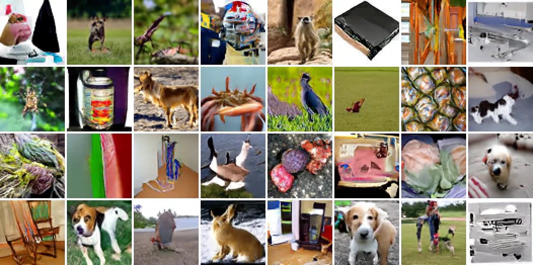
TL;DR: A diffusion model at two levels. One network denoises a compact embedding and the pixels, so it learns visual representations and generates images without labels, trained by denoising alone.
Representations learned by reconstructing, denoising or generating the image still trail those of non-generative self-supervised learning (SSL) methods. An image's exact color and framing are stochastic details that vary among images with the same content. A representation trained to reproduce the image is pushed to encode these details. Recognition, in contrast, benefits from invariance to them.
A diffusion model at two levels
DEM generates the representation and the image separately, within one network and with one denoising objective. In representation space, it denoises the embedding of an image given another view of the same image. In pixel space, it generates the image that this embedding describes. The network is one shared backbone, a Transformer, with two small heads on it. The embedding denoiser works at the embedding level, and the pixel head works at the pixel level.
Training
Each training step takes three views of one image. The teacher, an exponential moving average (EMA) of the network, embeds a clean view into the target. At the embedding level, the backbone reads the noised view, and the embedding denoiser recovers the target from a noisy copy of it (loss 1). At the pixel level, the backbone reads a noisy copy of the image with the target as its condition, and the pixel head predicts the image (loss 2).
Inference
After training, the teacher is no longer used. The Vision Transformer's features of an image are its representation, and no head is needed. To generate without labels, the embedding denoiser first samples an embedding from noise with no view, and the Vision Transformer and pixel head then draw the image given it. Given only a crop, the embedding denoiser samples several embeddings that fit the crop, and the pixel head draws one image for each.
Noise-map views
Masking and cropping amount to full noise on some patches. A single noising process, which sets a noise level for each patch, can thus produce both the views of SSL and the noisy images of diffusion. DEM draws all its inputs from this process, so its two tasks train on the same inputs. In training, the student sees a noised view (noise combined with a mask), the teacher a clean view, and the pixel pass a noised image (the whole image at one noise level).
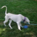
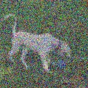
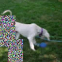
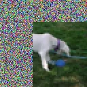
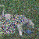
cleanfull noise
Asymmetric noise schedules
The embedding is denoised mostly near full noise, close to the SSL task where semantics are learned, and the pixels at lower noise, where the stochastic details are drawn.
The full-noise special case
Conceptually, joint-embedding SSL methods are a special case of DEM. These methods train a network to predict the embedding of one view of an image from another view. Suppose this network also receives a noisy copy of the embedding it predicts. If the copy is pure noise, it carries no information, and the task is unchanged. Prediction is thus view-conditioned embedding denoising at full noise. At lower noise, DEM learns the distribution that prediction reduces to its mean.
Lower noise (DEM). The copy still carries information.
Results
| DEM | Baseline | |
|---|---|---|
| Linear probe | 77.2% | 74.5% (DINOv2) |
| k-NN | 69.9% | 72.5% (DINOv2) |
| FID-50k without labels | 19.5 | 12.3 (RCG, three separate models) |
| Class-conditional FID-50k | 14.5 (1% of labels) | 12.4 (JiT, all labels) |
ImageNet-100, 64x64, ViT-S/8, 100k iterations, FID-50k. DINOv2 at the same training length. DEM has the higher linear probe and the lower k-NN accuracy. RCG trains three separate models. For class-conditional generation, DEM uses a linear probe fit on 1% of the labels, against class-conditional JiT trained on all labels.
One embedding, many images
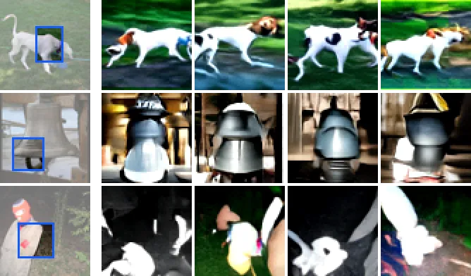
The embedding sets the content of the image, and the pixel noise supplies the stochastic details it leaves out.
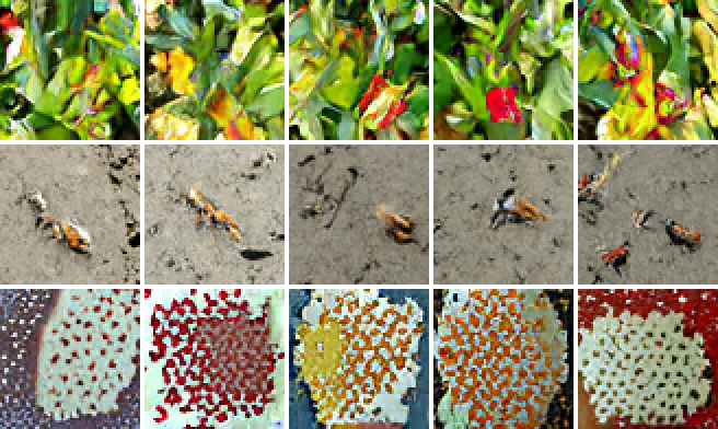
One sampled embedding per row, with varied pixel noise.
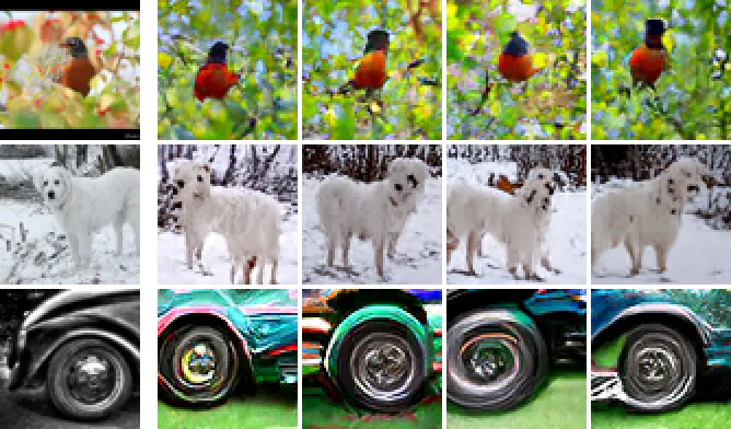
A validation image and samples from its embedding.
Completion and in-painting
DEM completes crops and in-paints without training for either.
Each image is decoded from an embedding sampled given the blue crop.
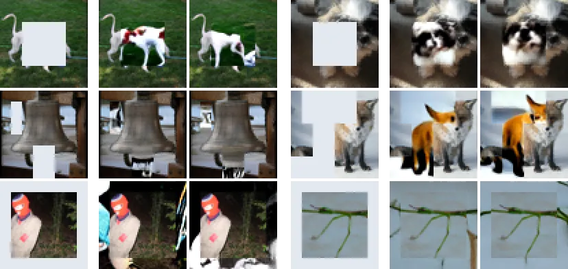
A hole, blocks and out-painting, with two samples each.
How DEM was built
We developed DEM through a speedrun in the style of modded-nanogpt. Every run trains for 20k iterations at batch size 512 on ImageNet-100 at 64x64 with a ViT-S/8, and changes one component of the current best model. Two numbers decide its fate, the linear probe and FID-5k without labels. Before launch, each change is written into the project journal with its hypothesis, its predicted effect and numeric bars for success and refutation. Seed 0 nominates a change and seed 1 confirms it. A change sets a record when its two-seed mean improves one metric by more than the seed spread (1.0 probe points or 2.5 FID) without the other getting worse by more than its spread.
The authors set the initial idea and the changes of direction. AI agents implemented candidate changes, launched the runs, compared each outcome with the prediction recorded before launch, and proposed the next experiments. Because this process adds components quickly, we paused periodically to simplify the model, removing what the central claim did not need. A removal was kept when both metrics stayed level.
| Record | Date | Probe | FID-5k |
|---|---|---|---|
| Joint model, pixel loss on the embedding denoiser | 9 Oct | 52.6% | 95.4 |
| Noise as a view | 16 Oct | 60.3% | 66.5 |
| Muon optimizer | 17 Oct | 67.7% | 63.1 |
| Asymmetric noise schedules | 19 Oct | 70.5% | 58.1 |
| Snapshot v2, adopted sampler | 26 Oct | 70.53% | 42.76 |
| Pixel pass as a view of the patch term | 3 Nov | 70.65% | 39.85 |
Selected records, two-seed means, 20k iterations, FID-5k without labels. The last two rows use the adopted sampler (guidance on an interval), which lowered the FID of the 20 October model from 59.4 to 46.1 without retraining.
Representation and generation mostly improve together. Across the 253 runs with the earlier sampler, a higher probe goes with a lower FID (Spearman −0.69), and across the 171 runs with the adopted sampler the correlation is −0.51. Single changes are less predictable. Among the 231 runs that modify a base configuration under the earlier sampler, the changes in the two metrics correlate at only −0.22.
A 20k record can fail at 100k. Eight local crops set a 20k record three times. On snapshot v2 they raised the two-seed probe from 70.53 to 72.08 at level FID. At 100k the run became unstable after 44k and finished at a probe of 75.54, below v2's 76.06. A 20k record now enters the model only after a 100k check.
Generation may help the representation with training. At 20k, removing the pixel loss raises the probe from 70.53 to 72.93 (two seeds). At 100k the sign reverses, and without the pixel loss the probe reaches 71.44 against 75.66 for seed 0 of the matching DEM run (the Results numbers are two-seed means). This is a single seed, so we treat it as a hypothesis until the second seed finishes.
BibTeX
@misc{awal2026dem,
  title  = {Denoising Embedding Models Are Generative Self-Supervised Learners},
  author = {Awal, Rabiul},
  year   = {2026}
}